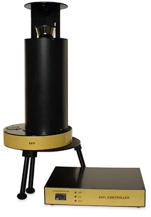
Method for Calibration of SATI Instruments

Introduction

The cross-calibration and testing of the airglow optical instruments are one of the goals of the developed NATO CLG and INTAS projects. The implementation of this task is also connected to making a low-cost laboratory facility for calibration and testing.

In this paper we present a calibration method for the SATI instruments used in the calibration of SATI-3SZ in Stara Zagora station. The suggested scheme is an alternative to the flat-field calibration by an integrating photometric sphere applied so far [1]. The exposed approach adheres to the specified requirements during technical implementation as well as to mobility.

Design of the method

The SATI-3SZ calibration includes two stages:

• Determination of the SATI responsivity for all working fields with input aperture, equally filled by homogeneous spectral emission.
• Attachment of the so determined flat-field to a radiometric specimen, calibrated in absolute energetic units.

Several laboratory settings have been made for the realization of the first stage:

1. The SATI calibration follows the optical scheme suggested by Canadian specialists from the Centre for Research in Earth and Space Science (CRESS), York University in Toronto, and is shown in the figure below. A light source illuminates a flat, diffuse reflecting white screen. The scattered light is reflected by the white ring put around the instrument's body towards the concave hemispheric surface and falls within the instrument's field of view.

   

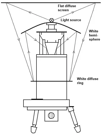
   This scheme has one important disadvantage. It does not ensure equal illuminance along the whole SATI field of view. Therefore, the results of this setting are accepted as insufficiently correct.

2. SATI-3SZ calibration by a photometric integrating sphere. Due to the specific construction of the sphere we used and the particular illumination scheme (four small halogen lamps arranged in a cross-like way near the sphere inlet), equal luminance of the scattering surface is not yet guaranteed. Precise measurement of the brightness in the radial direction was not performed, which is a disadvantage of the setting. Most integrating spheres are adapted for photometric instrumentation with a central, comparatively small field of view, while the instruments of the SATI or MORTI (Mesopause Oxygen Rotational Temperature Imager) [3] type have an angular field of view with external limits, reaching up to 70°. The last fact raises new strict requirements for the luminance homogeneity of the calibrating spherical surface as well as for the quality of the reflecting coating.

   

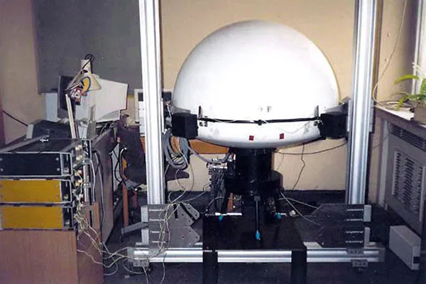
   The results obtained by the integrating sphere method are compared to the results calculated in our methodology, described in the next section. The relative difference is no more than 2%. Yet, this method requires high-cost and complex laboratory equipment as well as lacks any portability.

A method using a flat scattering surface

Our method uses a flat scattering surface. It has several advantages compared to the previous methods and is very suitable for the cross-calibration of the separate instruments operating around the world. The setting scheme is shown in the figure below.

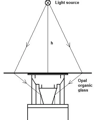
A point-like light source S is located at a distance h (in our case 1500 mm) along the optical axis over the SATI and illuminates a flat scattering screen fixed on top of the instrument. The considerations for the selection of a flat surface are the following:

Due to the specific path of the light rays for the SATI instrument, the separate light beams, forming different falling angles to the interference filter, see the flat surface always under the same angle. The parallel light beams falling on the filter come out of virtual point sources located along the radii of the input field stop, in the front focal plane of the Fresnel lens. These virtual point sources, on their part, are formed by light beams, equal in angular distribution (between 26° and 34°), yet falling on the conic mirror at different heights. In other words, these beams are identical and only translated to one another. Therefore, it is not necessary for the scattering surface to be strictly Lambertian (The Lambertian surface has the property to scatter the light in different angular directions in a specific way, described by the cosine law of the angle to the normal of the surface. As a consequence, the brightness in different directions is measured equal).

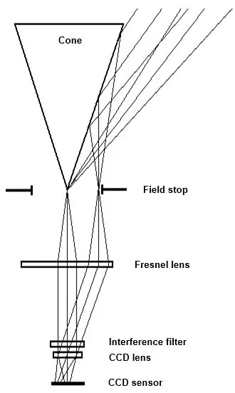
Each homogeneous white surface, sufficiently scattering the passing light, can be used as a diffuse material. In our implementation, we use a 4 mm thick white organic glass flat surface.

Another consideration in support of the flat scattering surface using the light scheme described so far is the well-known distribution of the illuminance E along a given radius in the instrument field of view, set out by Lambert’s cosine law: Е = I cos(θ) / L². In this way, the illumination E_P in point P at a distance r from the optical axis is:

E_P = I ⋅ h² / (r² + h²)^3/2

where I is the intensity of the light source, accepted for convenience to be equal to one. In practice, it should have a sufficiently high intensity value in order to provide the necessary signal-to-noise ratio (SNR) for a typical SATI exposition of 120 s. Because h is 1500 mm and r is almost ten times smaller, the above formula can be simplified using Taylor series, so we yield:

E_P ≈ I / h ⋅ (1 - 3/2 ⋅ r² / h²)

In our case, the maximum difference between the exact and approximate equation is no more than 0.05%.

Practical implementation

A small halogen lamp of 100 W is used as a light source. A round-shaped glass window, 2 mm thick and 10 mm in diameter, is fixed in front of it and is mat-coated on both sides. It plays the role of a point light source. As it is well known, the halogen lamp has a continuous emission spectrum with a shape close to the Planckian curve at Teff ≈ 3000 K. This provides a homogeneous spectrum in the whole operating range of the SATI instrument between 8645 Å and 8680 Å. The difference in the emission intensity between the two wavelengths is no more than 0.25%.

Approximately 250 images at a typical SATI exposition of 120 s are obtained and then averaged. Dark current images are recorded after every eight exposures. The flat-field obtained in this way should be numerically corrected because of the illuminance difference ΔE_P1,P2 of the two points P1 and P2 located at a distance of r1 and r2, respectively, along the SATI field of view. ΔE decreases with the increase of h. In the case of SATI-3SZ, h is 1500 mm, so ΔE is less than 1.5%.

The next figure shows that a virtual point source S' located at a distance x from the optical axis in the plane of the input field stop D is formed by the beams coming from the ring-shaped area on the diffusor, locked between the radia r1 and r2.

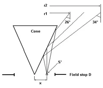
In our case:

r1(x) = 330⋅tan(26°) - 1.110⋅x
r2(x) = 330⋅tan(34°) - 1.203⋅x

Here r1, r2 and x are expressed in mm. On the other side, with known h, the total energetic flux of the source S' can be written as a definite integral taken from r1(x) to r2(x), or:

Ф(х) = ∫_r1(x)^r2(x) E(r) dr

For convenience, Ф(х) is expressed as a function of radius Rb of a given radial zone of the image in bins (in our case, one bin is composed of 2×2, i.e., four pixels from the CCD sensor) and hence, by the wavelength λ. For this purpose, the following equations are used:

x = 0.312⋅Rb
λ = λ₀ ⋅ (1 - Rb² / (µ² ⋅ (625² + Rb²)))^1/2

The numerical coefficients 0.312 and 625² are determined by the specific geometric parameters of SATI-3SZ, such as the focal length of the CCD camera lens, the focal length of the Fresnel lens and bin size. λ₀ and μ are the central wavelength of the interference filter and the effective refractive index, respectively. The experimentally obtained flat-field is corrected by the numerical coefficient Ф = Ф(λ) normalized to a unit towards its maximum value. The result is presented in the figure below. It is seen that this profile coincides very precisely with the profile obtained by the photometric sphere, and the relative difference between the two is no more than 2%. Probably, this is due to the inequality of the brightness of the sphere's surface, falling within the SATI field of view.

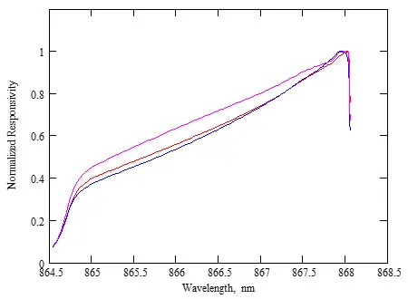
The second stage of the calibration process is the calculation of the SATI responsivity, expressed in absolute energetic units. It is performed using a Radiometer / Photometer Model 730A, Optronic Laboratories Inc. set in radiometric mode and equipped with a radiometric filter. The receiver measures the energetic brightness in W/cm2•sr. The filter ensures the constancy of the radiometric detector responsivity function in the range from 480 nm to 1000 nm with an accuracy of ±5%. The brightness of the diffusor is determined in 10 points located in a circle with a radius of 185 mm and then is averaged. It is taken into account that the quantity of energy registered from the radiometric detector can be expressed as an integral of the product of the detector's spectral responsivity and the spectral profile of the light source (we accept that the source emits as a black body with an effective temperature of 3000 K). SATI has a frequency range much narrow (8645 Å – 8680 Å) so the energy accepted by the instrument is about 120 times less than the one measured by the radiometer. The average responsivity obtained is 131 R/nm per ADU/s, where ADU is an analog-to-digital unit or simply the count. The last obtained SATI-3SZ profile, expressed in ADU•nm/R•s for a given wavelength λ, is shown in the figure below.

Conclusion

One possible source of inaccuracies in the proposed method could be the inhomogeneity of the diffuse material, which can be determined experimentally and corrected if necessary. Another source of errors could be the inaccurate centering of the light source relative to the optical axis of the SATI instrument. As final conclusions, the following observations can be made:

• The presented method can produce high precision in the flat-field calibration of instruments of the SATI–MORTI type. At h = 1500 mm, the difference in the total energetic fluxes forming the two final parallel beams and falling on the interference filter at 0° and 11°, respectively, is about 0.4%. After a numerical correction, the precision of the obtained flat-filed profile is not lower than 0.1%. The difficulties of achieving better accuracy are probably determined mostly by the inhomogeneity of the scattering material used for the calibration and also by the spectral characteristics of the light source. An important advantage of the suggested method is its technical simplicity and especially its mobility. The latter is essential for cross-calibration of the SATI–MORTI instruments operating at different geographic locations.

• The obtained flat-field shows the instrument's responsivity to a continuous spectrum. The signal received by SATI is a sum of a discrete spectrum (the six emission pares of (0-1) branch of the O₂ airglow atmospheric band system), overlayed on a continuous spectral homogeneous background. The calculated flat-field is actually the SATI responsivity towards this background. Due to the spectral character of the instruments of this type, in the above-described calibration procedure, the instrument's responsivity for discrete, spectrally narrow lines (the so-colled Point Spread Function, PSF) remains unknown. PSF plays a key role when the absolute rotational temperatures should be calculated.

  The form of the spectral profile of the instrument PSF is of primary significance for the synthetic spectra convolution. Small changes in it produce different rotational temperatures. So, we must calculate the spectral responsivity of the instrument with high-enough accuracy. An important peculiarity is that the characteristic type of the temperature course for a given night of observation remains the same and is only transferred by absolute value. We suggest several approaches for the solution to this problem. The first one (more precise) requires spectral calibration [2]. For this, the scattering surface is illuminated by a light source (precise monochromator with the linewidth of about 0.1 nm or a laboratory high-coherence laser), emitting in a spectral range sufficiently narrow compared to the line profile of the interference filter. It is necessary to take with sufficient precision the SATI's PSF at least in two finite points of the working spectral interval between 8645 Å and 8680 Å.

  The other approach is based on the assumption that the instrument's responsivity to the discrete spectrum is sufficiently close to the responsivity towards the continuous background. Thus, in the data processing, only the above-described flat-field will be applied. The data received by the SATI instrument should be matched to more precise ones obtained by other methods and equipment, for example, by Lidar systems.

  The third one consists of the PSF restoring with known input and output signals. Let the rectangular spectral signal f(λ) is an input function for the system, and the flat-field profile g(λ) is its image. Therefore, since the system is linear, the relationship between f(λ) and g(λ) is given by a convolution equation:

  g(λ) = f(λ) ∗ PSF(λ)

  However, there is one difficulty. The system is linear, but PSF changes on the SATI image plane between 8645 Å and 8680 Å. In other words, the system operator A is not commuting with the translation operator T:

  A[T[f(λ)]] ≠ T[A[f(λ)]]

  The solution to the above problem will be a subject of future work.

Also, in the future, the spectral profile of the light source will be measured with high-enough accuracy. The whole flat-field calibration setting will be realized in a compact mobile version.

Reference

1. Sargoytchev S., Brown S., Solheim B., Cho Y., Shepherd G., Lopez-Gonzalez M. Spectral airglow temperature imager (SATI) – a ground-based monitor of mesosphere temperature, Applied Optics, 2004.
2. Shepherd G. Spectral imaging of the atmosphere, International Geophysics Series, Vol. 82, 2002.
3. Wiens R., Zhang S., Peterson R., Shepherd G. MORTI: a mesopause oxygen rotational temperature imager, Planet. Space Sci., Vol. 39, No. 10, pp. 1363-1375, 1991.

An early version of this report was presented at the Joined NATO-CLG/INTAS Workshop Investigation of Regional Scale Atmospheric Motions and their Influence on the Mesosphere/Thermosphere/Ionosphere Region, September 6-10, 2004, Granada, Spain.